News

Colin Jones¹, Robin Smith², Spencer Liddicoat³, Andy Wiltshire³, Jeremy Walton³, Steve Rumbold² and Lee de Mora⁴

¹NCAS, University of Leeds, ²NCAS, University of Reading, ³Met Office, ⁴Plymouth Marine Laboratory.

Introduction and experiment protocol

We have designed a coupled Earth system model (ESM) experiment protocol for investigating climate risks at different levels of Global Warming (GWL) and associated with different magnitudes and duration of global warming overshoot (e.g. exceeding 2°C above pre-industrial (PI) values). We will use this protocol to investigate the risk, mechanisms behind, and subsequent impacts, of abrupt change in the TerraFIRMA focus phenomena; ice sheets, tropical forests and marine ecosystems, as well as for assessing the reversibility of any triggered abrupt changes. We will further use the experiments to assess social and environmental impacts arising from long-term stabilization of global climate at different GWLs, from overshooting key GWL targets, and the potential reversibility of such impacts if the Earth’s climate is cooled back to present-day or PI temperatures, sometime after warming stabilization. In this article we outline the experiment protocol (termed the TerraFIRMA Overshoot protocol, or TF-OS), present some initial results from TF-OS using a specific configuration of UKESM1.1 [1], and outline a timetable for making the TF-OS simulation data available to TerraFIRMA scientists and, more broadly, to the UK research community.

The TF-OS protocol is designed to produce a common rate of global mean surface warming (~0.2°C per decade) for any participating ESM, starting from its own pre-industrial (piControl) simulation. ESMs are run in CO₂-emission mode, with a constant rate of CO₂ emissions (mimicking anthropogenic emissions), allowing the model’s carbon cycle to determine the fraction of emitted CO₂ that remains in the atmosphere to the warm the planet, versus the fraction taken up by the model terrestrial or marine carbon sinks. Assuming a linear relationship between cumulative carbon emissions and global warming, as suggested by the transient climate response to cumulative emissions of CO₂ (TCRE, [2]), groups can use the TCRE value of their model to impose a constant CO₂ emission rate that generates a warming of ~0.2°C per decade. For UKESM1.1 this corresponds to a CO₂ emission rate of +8GtCyr^-1. We name this phase of the TF-OS protocol, the ramp-up phase.

Based on a 30-year running mean of simulated global mean surface air temperature (GSAT), we identify dates in the ramp-up run when different global warming level (GWL) are exceeded (e.g. 1.5 or 2°C above PI values from the parallel piControl run). At these dates we set CO₂ emissions to zero (i.e. net-zero anthropogenic emissions) and continue the run. We name this phase the zero emission or stabilization phase and envisage a near zero change in GSAT over this period. At designated timepoints into the warming stabilization run (e.g. after 50 and 200 years) we apply negative CO₂ emissions to the model (i.e. CO₂ is actively removed from the model atmosphere), initially sampling rates equal to, and half of, the positive ramp-up emission rate (i.e. -8GtCyr^-1 or -4GtCyr^-1). We name this the ramp-down phase. During the ramp-down we again identify when different GWL are passed (on the global cooling pathway) and repeat zero-emission, stabilization runs at these GWLs. We apply negative CO₂ emissions until the model climate has cooled back to its reference PI value and then set CO₂ emission to zero, resulting in a second piControl simulation, started from the end of a given ramp-up, warming stabilization, ramp-down pathway. To generate an ensemble of ramp-up, warming stabilization (at different GWLs) and ramp-down runs, we initiate a new ramp-up simulation every ~50 years along the reference piControl simulation. Figure 1 illustrates the TF-OS protocol.

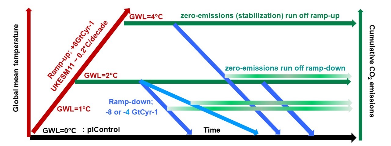
Figure 1: The TF-OS experiment protocol. The black line shows the piControl run, from which a ramp-up run is started (red line) with a CO₂ emission rate (GSAT warming rate) of +8GtCyr^-1 (0.2°C per decade). At different GWLs in the ramp-up, zero emission (stabilization) runs are started (green lines) and at different points into these runs, ramp-down (negative CO₂ emission) runs are started (blue lines). Zero emission runs can also be initiated off the ramp-down runs at different GWLs and at PI conditions.

Using this protocol, we can sample different GWLs and lengths of warming stabilization before ramp-down occurs, initializing stabilization runs from both ramp-up and ramp-down phases. The combination of these runs, phrased with respect to the rate, level and duration of global warming and cooling, (at and above different GWL targets), allow us to study the impact of these factors on the abrupt change phenomena addressed in TerraFIRMA, and on any ensuing socio-economic/environmental impacts. We can further contrast impacts and abrupt change risks between different GWLs and duration of stabilization.

Initial results from the TF-OS protocol

We present some initial results from our experiment protocol, using a specific configuration of UKESM1.1, run in CO₂-emission mode with interactively coupled models for both the Antarctic and Greenland ice sheets. We refer to this configuration as eUKESM11_ice. Figure 2 (left panel) shows the global mean atmospheric CO₂ concentration in one ramp-up member (black line), with a near linear increase in atmospheric CO₂ associated with the constant +8GtCyr^-1 emission rate. The various coloured lines (following near constant CO₂ levels) show zero emission (stabilization) runs started from different GWLs, as listed in the figure legend. The sharply negative CO₂ concentration lines on figure 1 are from -8GtCyr^-1 negative emission runs, started either 50 or 200 years into a given (similarly coloured) stabilization run. Even though CO₂ emissions are zero in the stabilization runs, atmospheric CO₂ concentrations slowly decreases. This is due to an imbalance between the accumulating atmospheric CO₂ and the terrestrial and marine carbon stores (mainly the marine store), which results in a continuing flux of CO₂ from the atmosphere to the ocean for ~200 years after the start of the (longest 2°C) zero emission run (see right panel in figure 2, which shows the global mean flux of CO₂ from the atmosphere into the ocean, with the coloured stabilization runs asymptoting towards zero flux over 200+ years). The different atmospheric CO₂ time series, for similarly coloured stabilization runs (e.g. for GWL=1.5°C and 2°C), each start at slightly different CO₂ concentrations (but at the same GWL). This reflects each member starting from a different ramp-up run, themselves started 50 years apart along the piControl run and reflects internal variability in both the carbon cycle and GSAT in the piControl and individual ramp-up members.

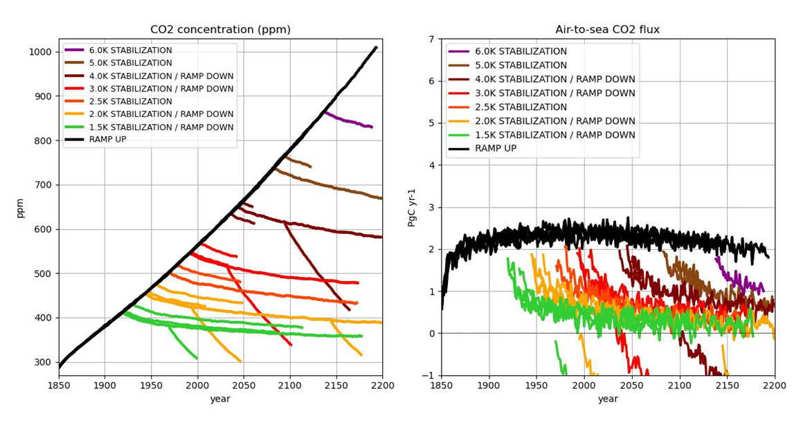
Figure 2: Left: Global mean atmospheric CO₂ concentration. Right: Global mean flux of CO₂ from the atmosphere to the ocean (positive values indicate flux into the ocean). Stabilization and ramp-down runs are coloured based on the GWL at which they branched from the ramp-up run. The three green stabilization lines and two yellow lines show different ensemble members (branching from different ramp-up runs) at the same respective GWL.

Figure 3 (left) plots the global mean, top of atmosphere (TOA), net radiative forcing and figure 3 (right) plots GSAT, in the various ramp-up, zero emission (stabilization) and ramp-down runs, as well as the piControl (black). By design, GSAT increases at ~0.2°C per decade in the ramp-up run. This is due to the increasing TOA net radiative imbalance that reaches ~2 Wm^-2 after ~150 years of +8GtCyr^-1 CO₂ emissions. In the zero-emission runs, the TOA net radiative forcing slowly decreases, primarily due to the decrease in atmospheric CO₂ concentrations, combined with longwave cooling of the planet. In terms of GSAT, this slow decrease in radiative forcing (a cooling tendency) is almost exactly balanced by the reappearance at the surface of heat sequestered into the ocean during the ramp-up phase (a warming tendency), resulting in a near constant GSAT in the zero emission runs.

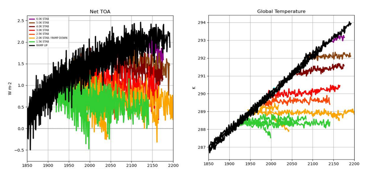
Figure 3. Left: Global mean TOA net radiation flux (positive downward). Right: Global mean surface air temperature. Runs colour coded as described in Figure 2.

Figure 4 shows the response of the Atlantic Meridional Overturning Circulation (AMOC) in the piControl (blue), ramp-up run (black) and various zero-emission (stabilization) runs. The AMOC transports a large amount of heat poleward in the near-surface Atlantic, with a deep return flow at depth connecting the north Atlantic to the Southern Ocean. The AMOC has shown periods of rapid weakening (near collapse) in paleo-observations [3], which are thought to be driven by large inputs of freshwater into the North Atlantic from neighbouring land, reducing surface ocean density and weakening deep ocean mixing, disrupting the overturning circulation [4]. The majority of CMIP5 and CMIP6 projections suggest the AMOC will decrease in strength in the future [5]. The eUKESM1.1_ice ramp-up also shows a weakening of the AMOC, with the piControl AMOC (~14Sv) weakening to ~9Sv after 250 years of ramp-up (or ~5°C global warming). In the majority of the zero emission (stabilization) runs the AMOC decline stabilizes but shows no sign of recovering strength. The ramp-down runs have not yet run for sufficiently long time to detect a reliable signal as to whether the AMOC will recover or remain at its weaker (zero emission) strength.

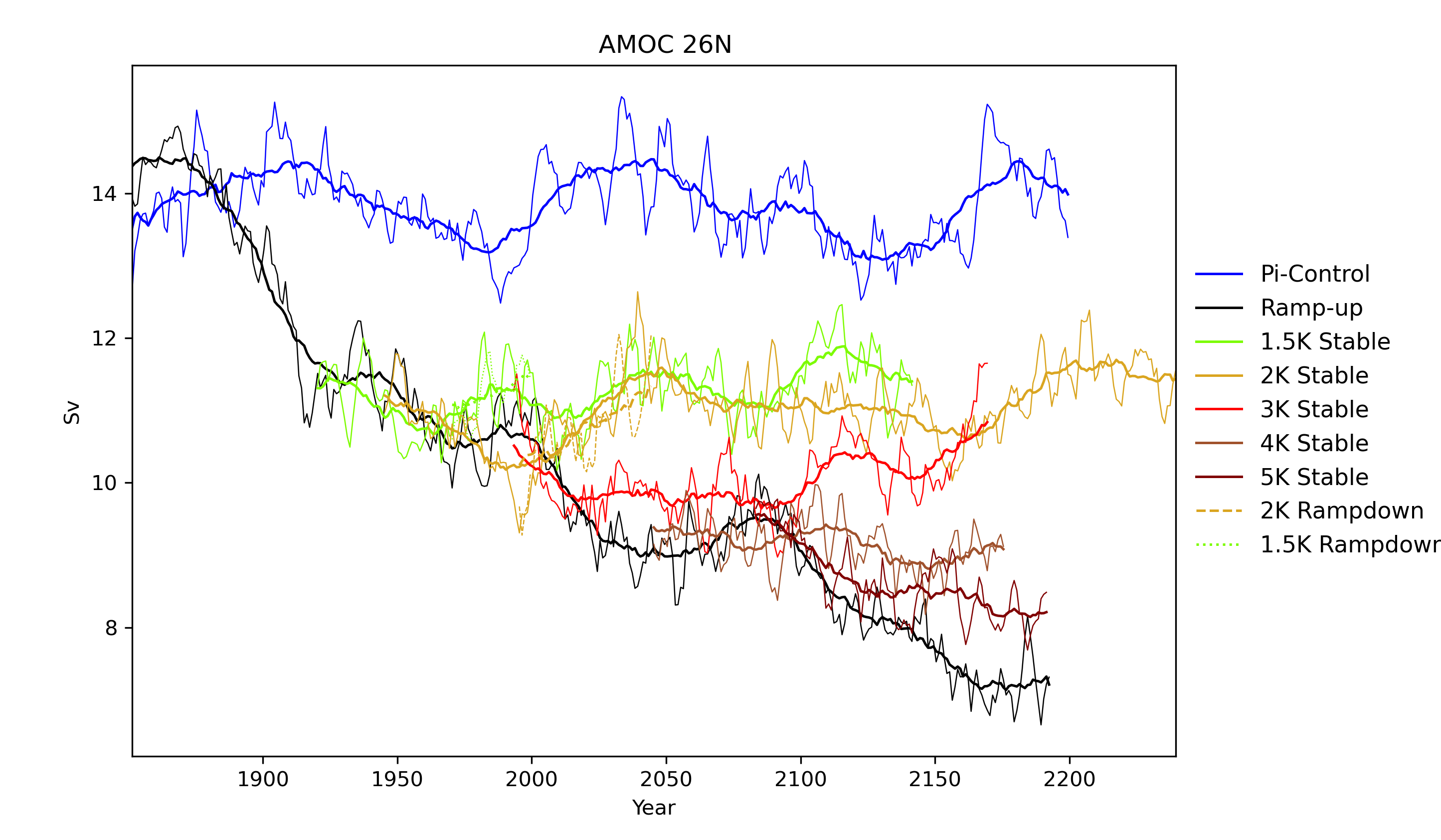
Figure 4: AMOC strength at 26°N in Sv in the piControl (blue), ramp-up (black) and various GWL zero emission runs and -8GtCyr-1 ramp-down runs. Colours in the legend indicate the GWL values. Thin lines show a 5-year running mean of AMOC strength, while thick lines are a 30-year running mean.

Finally, figure 5 shows ice mass loss from the Greenland (left panel) and Antarctic (right panel) ice sheets, expressed as metres of potential global sea level rise (NB for Antarctic mass loss we include mass lost from already-floating ice shelves that will not directly contribute to sea-level itself). The Greenland ice sheet slowly gains mass in the piControl but loses mass at an ever-accelerating rate in the ramp-up run. Stabilizing global temperature at any given GWL stabilizes only the rate of mass loss not the ice sheet itself, which continues to steadily lose mass with a more linear trend. The picture for the Antarctic ice sheet is more complex. This loses mass in every simulation, including the piControl. We initialise the model with an unstable West Antarctic sector, as observed in the modern ice sheet, and this part of the ice sheet continues to thin and retreat in all these runs. Below around 4°C of warming, the ramp-up run shows less mass loss than the piControl because the warmer air results in more snowfall whilst still remaining too cold for summer melt to dominate the surface mass balance. The ramp-up run shows two noticeable accelerations in mass loss. The first is around the 4°C GWL where the ocean density in the Ross sector crosses a threshold and warm water floods the cavity under the ice shelf, leading to greatly increased basal melting. The second acceleration comes between 5 and 6°C, where a similar process starts to melt the massive Filchner-Ronne ice shelf. Stabilising above the 2.5°C GWL does not prevent the Ross shelf regime shift occurring, but Filchner-Ronne melting only happens above the 5°C GWL.

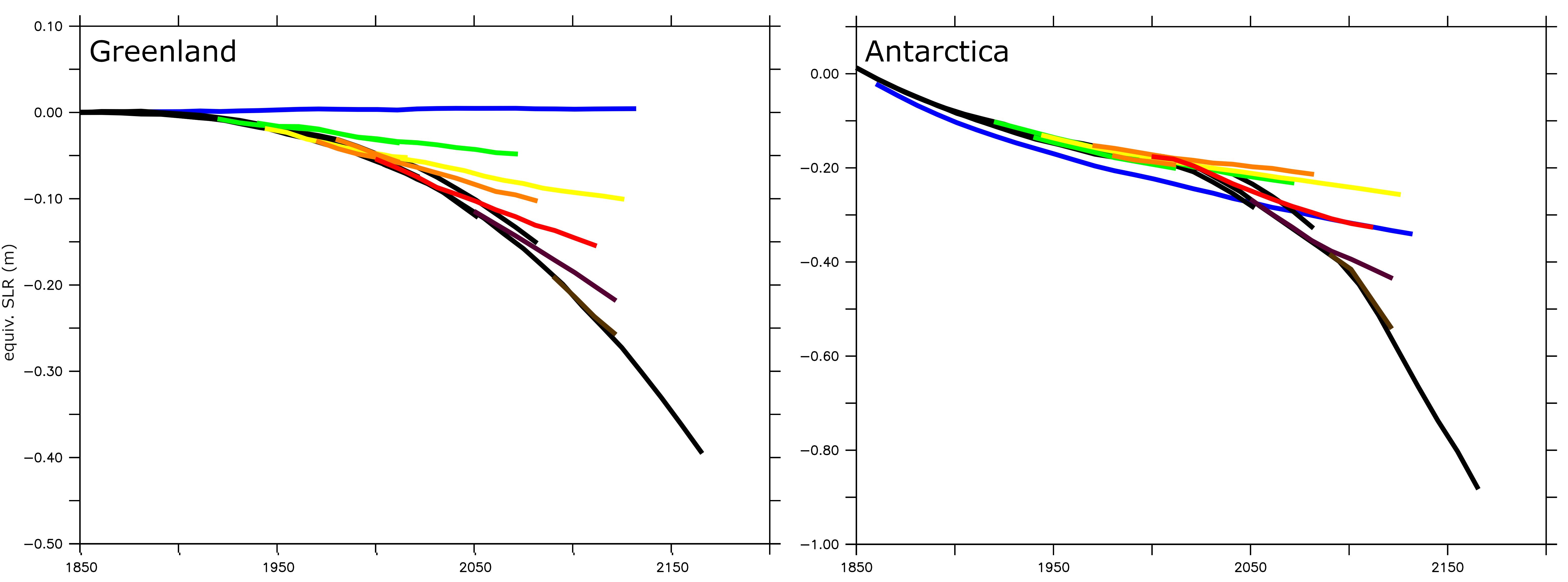
Figure 5: Change in ice mass (equivalent metres of sea-level contribution) from the interactive ice sheets in TF-OS simulations. Left: Greenland; right: Antarctica. Blue: piControl; black: ramp-up. Other colours are stabilisation at different GWLs: green 1.5K; yellow 2K; orange 2.5K; red 3K; violet 4K; brown 5K.

Data conversion and data availability

We plan to initially run for 4 ramp-up members (with initial conditions separated by 50 years along the piControl simulation) using +8GtCyr^-1 CO₂ emissions. From each ramp-up member we will branch four zero-emission members for GWLs = 1.5, 2, 3, 4 and 5°C. 50 and 200 years into each zero-emission GWL run we will branch off ramp-down runs using -8GtCyr^-1 emissions. Additional ramp-down runs at -4GtCyr^-1 will be made from year 50 of the respective zero emission runs. Finally, we will repeat selected zero emission runs branched off the ramp-down runs (e.g. at GWL = 2 and 1.5°C). At least one zero emission member, for each GWL, will be run for 700 years. We aim to CMORize (e.g. in standard CMIP6 output format) an initial set of these runs, sampling the piControl and one ramp-up, zero emission and ramp-down member for both GWL =1.5 and 2°C, in January 2024, and make this data available to project members via the JASMIN platform. The full set of TF-OS data should be available to project members from ~April 2024. We will review these simulations at the TerraFIRMA General Assembly (May 2024), develop an analysis and exploitation plan across the project, and decide if more simulations are required. We aim to make the TF-OS data available more broadly, to collaborators in the UK research community, likely from late summer 2024.

References

• [1] Mulcahy J.P. et al 2023. https://doi.org/10.5194/gmd-16-1569-2023
• [2] MacDougall, A.H. 2016. https://doi.org/10.1007/s40641-015-0030-6
• [3] Clark, P. et al. https://doi.org/10.1038/415863a
• [4] McManus, J. et al. https://doi.org/10.1038/nature02494
• [5] Weijer, W. et al. 2020. https://doi.org/10.1029/2019GL086075